量子隐形传态
本节演示了量子隐形传态。我们首先使用Qiskit的内置模拟器来测试我们的量子电路,然后在真实的量子计算机上进行实验。
1. 概述
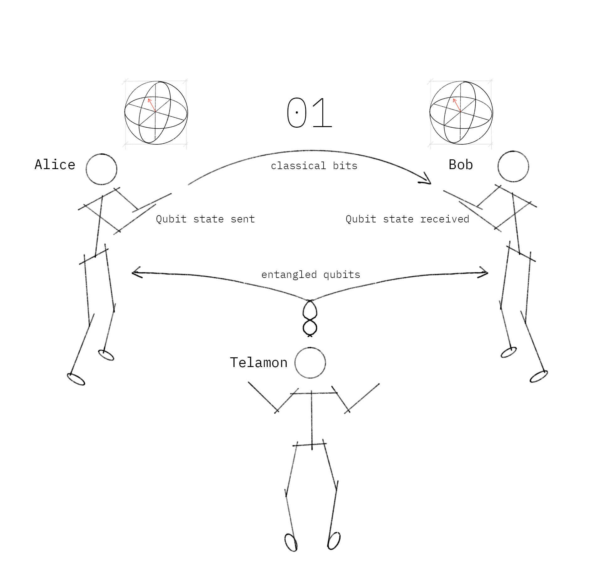
Alice想给Bob发送量子信息。具体来说,假设她想发送量子比特状态 \ket{\psi} = \alpha\ket{0} + \beta\ket{1} 。这需要将 α 和 β 的信息传递给Bob。
量子力学中存在一个定理:你不能简单地对一个未知的量子态进行精确的复制。这被称为不可克隆定理。因此,我们可以看到,Alice不能简单地生成|ψ⟩的副本并将该副本交给Bob。我们只能复制经典态(不是叠加态)。
然而,通过利用两个经典比特和一个纠缠的量子比特对,Alice可以将她的状态 \ket{\psi} 传输给Bob。我们称之为隐形传态,因为到最后,Bob将有 \ket{\psi} ,而Alice不再拥有。
2. 量子隐形传态协议
为了传输量子比特,Alice和Bob必须使用第三方(Telamon)发送一个纠缠的量子比特对。然后Alice对她的量子比特执行一些操作,通过经典通信信道将结果发送给Bob, Bob随后在他的一端执行一些操作以接收Alice的量子比特。
我们将在下面描述一个量子电路上的步骤。在这里,没有量子比特被实际“发送”,你只需要想象一下那部分!
首先,我们设置了会话:
# Do the necessary imports

import numpy as np

from qiskit import QuantumCircuit, QuantumRegister, ClassicalRegister

from qiskit import IBMQ, Aer, transpile, assemble

from qiskit.visualization import plot_histogram, plot_bloch_multivector, array_to_latex

from qiskit.extensions import Initialize

from qiskit.ignis.verification import marginal_counts

from qiskit.quantum_info import random_statevector
然后创建我们的量子电路:
## SETUP

# Protocol uses 3 qubits and 2 classical bits in 2 different registers

qr = QuantumRegister(3, name="q") # Protocol uses 3 qubits

crz = ClassicalRegister(1, name="crz") # and 2 classical bits

crx = ClassicalRegister(1, name="crx") # in 2 different registers

teleportation_circuit = QuantumCircuit(qr, crz, crx)
步骤1
第三方Telamon创建了一对纠缠量子比特,一个给Bob,一个给Alice。
Telamon创造的是一种特殊的对,叫做贝尔对(Bell pair)。在量子电路语言中,在两个量子比特之间创建贝尔对的方法是首先使用Hadamard门将其中一个量子比特转移到x基( \ket{+} 和 \ket{-} ),然后将CNOT门应用到由x基中的一个量子比特控制的另一个量子比特上。
def create_bell_pair(qc, a, b):

"""Creates a bell pair in qc using qubits a & b"""

qc.h(a) # Put qubit a into state |+>

qc.cx(a,b) # CNOT with a as control and b as target
## SETUP

# Protocol uses 3 qubits and 2 classical bits in 2 different registers

qr = QuantumRegister(3, name="q")

crz, crx = ClassicalRegister(1, name="crz"), ClassicalRegister(1, name="crx")

teleportation_circuit = QuantumCircuit(qr, crz, crx)

## STEP 1

# In our case, Telamon entangles qubits q1 and q2

# Let's apply this to our circuit:

create_bell_pair(teleportation_circuit, 1, 2)

# And view the circuit so far:

teleportation_circuit.draw()

假设在他们分开之后,Alice拥有 q_1 ,Bob拥有 q_2 。
步骤2
Alice对 q_1 应用CNOT门, q_1 由 \ket{\psi} 控制(她试图发送给Bob的量子比特)。然后Alice将Hadamard门应用于 \ket{\psi} 。在我们的量子线路中,Alice试图发送的量子比特( \ket{\psi} )是 q_0 :
def alice_gates(qc, psi, a):

qc.cx(psi, a)

qc.h(psi)
## SETUP

# Protocol uses 3 qubits and 2 classical bits in 2 different registers

qr = QuantumRegister(3, name="q")

crz, crx = ClassicalRegister(1, name="crz"), ClassicalRegister(1, name="crx")

teleportation_circuit = QuantumCircuit(qr, crz, crx)

## STEP 1

create_bell_pair(teleportation_circuit, 1, 2)

## STEP 2

teleportation_circuit.barrier() # Use barrier to separate steps

alice_gates(teleportation_circuit, 0, 1)

teleportation_circuit.draw()

步骤3
接下来,Alice对她拥有的两个量子比特 q_1 和 \ket{\psi} 进行测量,并将结果存储在两个经典比特中。然后,她将这两个比特发送给Bob。
def measure_and_send(qc, a, b):

"""Measures qubits a & b and 'sends' the results to Bob"""

qc.barrier()

qc.measure(a,0)

qc.measure(b,1)
## SETUP

# Protocol uses 3 qubits and 2 classical bits in 2 different registers

qr = QuantumRegister(3, name="q")

crz, crx = ClassicalRegister(1, name="crz"), ClassicalRegister(1, name="crx")

teleportation_circuit = QuantumCircuit(qr, crz, crx)

## STEP 1

create_bell_pair(teleportation_circuit, 1, 2)

## STEP 2

teleportation_circuit.barrier() # Use barrier to separate steps

alice_gates(teleportation_circuit, 0, 1)

## STEP 3

measure_and_send(teleportation_circuit, 0 ,1)

teleportation_circuit.draw()

步骤4
Bob已经拥有量子比特q2,然后根据经典比特的状态应用以下门:
00 \rightarrow Do nothing
01 \rightarrow Apply X gate
10 \rightarrow Apply Z gate
11 \rightarrow Apply ZX gate
(注意,这种信息传递是纯粹经典的。)
# This function takes a QuantumCircuit (qc), integer (qubit)

# and ClassicalRegisters (crz & crx) to decide which gates to apply

def bob_gates(qc, qubit, crz, crx):

# Here we use c_if to control our gates with a classical

# bit instead of a qubit

qc.x(qubit).c_if(crx, 1) # Apply gates if the registers

qc.z(qubit).c_if(crz, 1) # are in the state '1'
## SETUP

# Protocol uses 3 qubits and 2 classical bits in 2 different registers

qr = QuantumRegister(3, name="q")

crz, crx = ClassicalRegister(1, name="crz"), ClassicalRegister(1, name="crx")

teleportation_circuit = QuantumCircuit(qr, crz, crx)

## STEP 1

create_bell_pair(teleportation_circuit, 1, 2)

## STEP 2

teleportation_circuit.barrier() # Use barrier to separate steps

alice_gates(teleportation_circuit, 0, 1)

## STEP 3

measure_and_send(teleportation_circuit, 0, 1)

## STEP 4

teleportation_circuit.barrier() # Use barrier to separate steps

bob_gates(teleportation_circuit, 2, crz, crx)

teleportation_circuit.draw()

瞧!在这个协议的最后,Alice的量子比特现在已经传送给了Bob。
3. 模拟量子隐形传态协议
3.1 我们将如何在量子计算机上测试该协议?
在本小节中,我们将以随机状态 \ket{\psi} (psi)初始化Alice的量子比特。这个状态将用一个初始化门在 \ket{q_0} 上创建。在本章中,我们使用函数random_statevector来为我们选择psi,但可以随意将psi设置为任何你想要的量子比特状态。
# Create random 1-qubit state

psi = random_statevector(2)

# Display it nicely

display(array_to_latex(psi, prefix="|\\psi\\rangle ="))

# Show it on a Bloch sphere

plot_bloch_multivector(psi)

让我们创建初始化指令,从状态 \ket{0} 创建 \ket{\psi} :
init_gate = Initialize(psi)

init_gate.label = "init"
(Initialize is technically not a gate since it contains a reset operation, and so is not reversible. We call it an ‘instruction’ instead). If the quantum teleportation circuit works, then at the end of the circuit the qubit \ket{q_2} will be in this state. We will check this using the statevector simulator.
3.2 使用模拟状态向量
我们可以使用Aer模拟器来验证我们的量子比特已经被传送了。
## SETUP

qr = QuantumRegister(3, name="q") # Protocol uses 3 qubits

crz = ClassicalRegister(1, name="crz") # and 2 classical registers

crx = ClassicalRegister(1, name="crx")

qc = QuantumCircuit(qr, crz, crx)

## STEP 0

# First, let's initialize Alice's q0

qc.append(init_gate, [0])

qc.barrier()

## STEP 1

# Now begins the teleportation protocol

create_bell_pair(qc, 1, 2)

qc.barrier()

## STEP 2

# Send q1 to Alice and q2 to Bob

alice_gates(qc, 0, 1)

## STEP 3

# Alice then sends her classical bits to Bob

measure_and_send(qc, 0, 1)

## STEP 4

# Bob decodes qubits

bob_gates(qc, 2, crz, crx)

# Display the circuit

qc.draw()

利用从aer模拟器中得到的状态向量,我们可以看到, \ket{q_2} 的状态与我们上面创建的 \ket{\psi} 的状态相同,而 \ket{q_0} 的状态和 \ket{q_1} 的状态已经坍缩为 \ket{0} 或 \ket{1} 。状态 \ket{\psi} 已经从量子比特0传送到量子比特2。
sim = Aer.get_backend('aer_simulator')

qc.save_statevector()

out_vector = sim.run(qc).result().get_statevector()

plot_bloch_multivector(out_vector)

你可以多运行几次这个单元格来确定。你可能会注意到,量子比特0和1的状态会发生变化,但量子比特2始终处于 \ket{\psi} 状态。
3.3 使用模拟计数
量子隐形传态被设计为在两方之间发送量子比特。我们没有硬件来证明这一点,但是我们可以证明门在单个量子芯片上执行正确的转换。这里我们再次使用aer模拟器来模拟如何测试我们的协议。
在真正的量子计算机上,我们将无法对状态向量进行采样,因此如果要检查我们的隐形传态电路是否工作,我们需要做的事情略有不同。Initialize指令首先执行重置,将我们的量子比特设置为状态 \ket{0} 。然后应用门将我们的 \ket{0} 量子比特转换为状态 \ket{\psi} :
由于所有的量子门都是可逆的,我们可以使用以下方法找到这些门的逆:
inverse_init_gate = init_gate.gates_to_uncompute()
该操作具有以下性质:
为了证明量子比特 \ket{q_0} 已被传送到 \ket{q_2} ,如果我们在 \ket{q_2} 上进行反向初始化,我们期望确定地测量 \ket{q_0} 。我们在下面的电路中这样做:
## SETUP

qr = QuantumRegister(3, name="q") # Protocol uses 3 qubits

crz = ClassicalRegister(1, name="crz") # and 2 classical registers

crx = ClassicalRegister(1, name="crx")

qc = QuantumCircuit(qr, crz, crx)

## STEP 0

# First, let's initialize Alice's q0

qc.append(init_gate, [0])

qc.barrier()

## STEP 1

# Now begins the teleportation protocol

create_bell_pair(qc, 1, 2)

qc.barrier()

## STEP 2

# Send q1 to Alice and q2 to Bob

alice_gates(qc, 0, 1)

## STEP 3

# Alice then sends her classical bits to Bob

measure_and_send(qc, 0, 1)

## STEP 4

# Bob decodes qubits

bob_gates(qc, 2, crz, crx)

## STEP 5

# reverse the initialization process

qc.append(inverse_init_gate, [2])

# Display the circuit

qc.draw()

我们可以看到在电路图上出现了inverse_init_gate,标记为disentangler。最后,我们测量第三个量子比特,并将结果存储在第三个经典比特中:
# Need to add a new ClassicalRegister

# to see the result

cr_result = ClassicalRegister(1)

qc.add_register(cr_result)

qc.measure(2,2)

qc.draw()

然后运行我们的实验:
t_qc = transpile(qc, sim)

t_qc.save_statevector()

counts = sim.run(t_qc).result().get_counts()

qubit_counts = [marginal_counts(counts, [qubit]) for qubit in range(3)]

plot_histogram(qubit_counts)

可以看到,我们有100%的机会在状态 \ket{0} 下测量 q_2 (直方图中的紫色条)。这是预期的结果,表明隐形传态协议已经正常工作。
4. 理解量子隐形传态
既然你已经完成了量子隐形传态的实现,现在是时候了解协议背后的数学原理了。
步骤1
量子隐形传态始于Alice需要将 \ket{\psi} = \alpha\ket{0} + \beta\ket{1} (一个随机量子比特)传输给Bob。她不知道量子比特的状态。为此,Alice和Bob接受了第三方(Telamon)的帮助。Telamon为Alice和Bob准备了一对纠缠量子比特。纠缠的量子比特可以用狄拉克符号表示为:
Alice和Bob各自拥有纠缠对中的一个量子比特(分别记为A和B),
这就创建了一个三量子比特系统,其中Alice拥有前两个量子比特,Bob拥有最后一个量子比特。
步骤2
现在,根据协议,Alice在她的两个量子比特上应用CNOT门,然后在第一个量子比特上应用Hadamard门。结果如下:
它们可以被分离并写成:
步骤3
Alice测量了前两个量子比特(她自己的),并将它们作为两个经典比特发送给Bob。她获得的结果总是四个标准基态 \ket{00}、\ket{01}、\ket{10}、\ket{11} 之一,且概率相同。
根据她的测量,Bob的状态将被投影到,
步骤4
Bob在接收到Alice的比特后,就知道他可以通过对曾经是纠缠对的一部分的他的量子比特进行适当的变换来获得原始状态 \ket{\psi} 。
他需要应用的变换如下:
经过这一步,Bob将成功重建Alice的状态。
5. 真实量子计算机上的隐形传态
5.1 IBM硬件和延迟测量
IBM量子计算机目前不支持测量后的指令,这意味着我们无法在真实硬件上运行当前形式的量子隐形传态。幸运的是,由于文献[1]第4.4章讨论的延迟测量原理,这并不限制我们进行任何计算的能力。该原理指出任何测量都可以推迟到电路的末端,即我们可以将所有的测量移动到末端,并且我们应该看到相同的结果。

尽早测量的任何好处都与硬件有关:如果我们能够尽早测量,我们可能能够重复使用量子比特,或减少量子比特处于脆弱叠加状态的时间。在这个例子中,量子隐形传态的尽早测量将允许我们在没有直接量子通信信道的情况下传输一个量子比特态。
当移动门允许我们在真实硬件上演示"隐形传态"电路时,需要注意的是,隐形传态过程(通过经典通道传输量子态)的好处丢失了。
我们将bob_gate函数重写为new_bob_gates:
def new_bob_gates(qc, a, b, c):

qc.cx(b, c)

qc.cz(a, c)
然后创建我们的新电路:
qc = QuantumCircuit(3,1)

# First, let's initialize Alice's q0

qc.append(init_gate, [0])

qc.barrier()

# Now begins the teleportation protocol

create_bell_pair(qc, 1, 2)

qc.barrier()

# Send q1 to Alice and q2 to Bob

alice_gates(qc, 0, 1)

qc.barrier()

# Alice sends classical bits to Bob

new_bob_gates(qc, 0, 1, 2)

# We undo the initialization process

qc.append(inverse_init_gate, [2])

# See the results, we only care about the state of qubit 2

qc.measure(2,0)

# View the results:

qc.draw()

5.2 执行
# First, see what devices we are allowed to use by loading our saved accounts

IBMQ.load_account()

provider = IBMQ.get_provider(hub='ibm-q')
# get the least-busy backend at IBM and run the quantum circuit there

from qiskit.providers.ibmq import least_busy

from qiskit.tools.monitor import job_monitor

backend = least_busy(provider.backends(filters=lambda b: b.configuration().n_qubits >= 3 and

not b.configuration().simulator and b.status().operational==True))

t_qc = transpile(qc, backend, optimization_level=3)

job = backend.run(t_qc)

job_monitor(job) # displays job status under cell
Job Status: job has successfully run
# Get the results and display them

exp_result = job.result()

exp_counts = exp_result.get_counts(qc)

print(exp_counts)

plot_histogram(exp_counts)
{‘0’: 894, ‘1’: 130}

正如我们在这里看到的,有一些测量结果为 \ket{1} 。这是门和量子比特中的误差引起的。相比之下,我们在本节前面部分中的模拟器的门中没有误差,并且允许无误差的传输。
print(f"The experimental error rate : {exp_counts['1']*100/sum(exp_counts.values()):.3f}%")
The experimental error rate : 12.695%
6. 参考文献
[1] M. Nielsen and I. Chuang, Quantum Computation and Quantum Information, Cambridge Series on Information and the Natural Sciences (Cambridge University Press, Cambridge, 2000).
[2] Eleanor Rieffel and Wolfgang Polak, Quantum Computing: a Gentle Introduction (The MIT Press Cambridge England, Massachusetts, 2011).
import qiskit.tools.jupyter

%qiskit_version_table
/usr/local/anaconda3/lib/python3.7/site-packages/qiskit/aqua/__init__.py:86: DeprecationWarning: The package qiskit.aqua is deprecated. It was moved/refactored to qiskit-terra For more information see <https://github.com/Qiskit/qiskit-aqua/blob/main/README.md#migration-guide>

warn_package('aqua', 'qiskit-terra')
版本信息
| Qiskit Software | Version |
| -----: | ----: |
| qiskit-terra | 0.18.0 |
| qiskit-aer | 0.8.2 |
| qiskit-ignis | 0.6.0 |
| qiskit-ibmq-provider | 0.15.0 |
| qiskit-aqua | 0.9.4 |
| qiskit | 0.28.0 |
| System information | |
| -----: | ----: |
| Python | 3.7.7 (default, May 6 2020, 04:59:01) [Clang 4.0.1 (tags/RELEASE_401/final)] |
| OS | Darwin |
| CPUs | 8 |
| Memory (Gb) | 32.0 |
Tue Aug 24 11:07:09 2021 BST